41 multiple data labels excel pie chart

Create a multi-level category chart in Excel - ExtendOffice 2. Select the data range, click Insert > Insert Column or Bar Chart > Clustered Bar.. 3. Drag the chart border to enlarge the chart area. See the below demo. 4. Right click the bar and select Format Data Series from the right-clicking menu to open the Format Data Series pane.. Tips: You can also double click any of the bars to open the Format Data Series pane. Multiple Data Labels on a Pie Chart | MrExcel Message Board Hello All, So I have a table with 8 rows and 3 columns. This table includes: Column 1 - shipment name Column 2 - shipment cost Column 3 - shipment weight I have created a pie chart from this table, which covers the first two columns. Displayed next to each slice is a label with the...

How to Create a Pie Chart in Excel - Smartsheet Enter data into Excel with the desired numerical values at the end of the list. Create a Pie of Pie chart. Double-click the primary chart to open the Format Data Series window. Click Options and adjust the value for Second plot contains the last to match the number of categories you want in the "other" category.

Multiple data labels excel pie chart

Pie Chart in Excel | How to Create Pie Chart | Step-by ... Step 1: Do not select the data; rather, place a cursor outside the data and insert one PIE CHART. Go to the Insert tab and click on a PIE. Step 2: once you click on a 2-D Pie chart, it will insert the blank chart as shown in the below image. Step 3: Right-click on the chart and choose Select Data. Pie Charts in Excel - How to Make with Step by Step Examples Task b: Add data labels and data callouts. Step 3: Right-click the pie chart and expand the "add data labels" option. Next, choose "add data labels" again, as shown in the following image. Step 4: The data labels are added to the chart, as shown in the following image. Change the format of data labels in a chart Tip: To switch from custom text back to the pre-built data labels, click Reset Label Text under Label Options. To format data labels, select your chart, and then in the Chart Design tab, click Add Chart Element > Data Labels > More Data Label Options. Click Label Options and under Label Contains, pick the options you want.

Multiple data labels excel pie chart. Add or remove data labels in a chart On the Design tab, in the Chart Layouts group, click Add Chart Element, choose Data Labels, and then click None. Click a data label one time to select all data labels in a data series or two times to select just one data label that you want to delete, and then press DELETE. Right-click a data label, and then click Delete. How to Create Multi-Category Charts in Excel ... Implementation : Step 1: Insert the data into the cells in Excel. Now select all the data by dragging and then go to "Insert" and select "Insert Column or Bar Chart". A pop-down menu having 2-D and 3-D bars will occur and select "vertical bar" from it. Select the cell -> Insert -> Chart Groups -> 2-D Column. Pie of Pie Chart in Excel - Inserting, Customizing - Excel ... Inserting a Pie of Pie Chart. Let us say we have the sales of different items of a bakery. Below is the data:-. To insert a Pie of Pie chart:-. Select the data range A1:B7. Enter in the Insert Tab. Select the Pie button, in the charts group. Select Pie of Pie chart in the 2D chart section. Create Multiple Pie Charts in Excel using Worksheet Data ... Microsoft Chart Object for Excel provides all the necessary properties and methods to create charts in your Excel workbook, efficiently. You can create charts on your worksheet or create "separate" sheets with the charts. All you need is data. 👉 Do you know you can create multiple Line Charts automatically using a Macro? Check out this ...

Add data labels and callouts to charts in Excel 365 ... Step #1: After generating the chart in Excel, right-click anywhere within the chart and select Add labels . Note that you can also select the very handy option of Adding data Callouts. Step #2: When you select the "Add Labels" option, all the different portions of the chart will automatically take on the corresponding values in the table ... Excel Pie Chart Multiple Labels Add or remove data labels in a chart. Excel Details: On the Design tab, in the Chart Layouts group, click Add Chart Element, choose Data Labels, and then click None.Click a data label one time to select all data labels in a data series or two times to select just one data label that you want to delete, and then press DELETE. Right-click a data label, and then click Delete. label lines in excel ... How to Combine or Group Pie Charts in Microsoft Excel Another reason that you may want to combine the pie charts is so that you can move and resize them as one. Click on the first chart and then hold the Ctrl key as you click on each of the other charts to select them all. Click Format > Group > Group. All pie charts are now combined as one figure. Plot Multiple Data Sets on the Same Chart in Excel ... Follow the below steps to implement the same: Step 1: Insert the data in the cells. After insertion, select the rows and columns by dragging the cursor. Step 2: Now click on Insert Tab from the top of the Excel window and then select Insert Line or Area Chart. From the pop-down menu select the first "2-D Line".

How to make a pie chart in Excel - ablebits.com Adding data labels to Excel pie charts. In this pie chart example, we are going to add labels to all data points. To do this, click the Chart Elements button in the upper-right corner of your pie graph, and select the Data Labels option. Additionally, you may want to change the Excel pie chart labels location by clicking the arrow next to Data ... Creating Pie Chart and Adding/Formatting Data Labels (Excel) Creating Pie Chart and Adding/Formatting Data Labels (Excel) Creating Pie Chart and Adding/Formatting Data Labels (Excel) How to make a pie chart with two sets of data in Excel - Quora Answer: A pie chart isn't meant to show two sets of data. The pie is 100% of the data and the slices are portions representing what part of the whole each category represents. What are you trying to convey with two datasets? Is it possible you want to make two pie charts side-by-side so people ca... Multiple data labels (in separate locations on chart) Running Excel 2010 2D pie chart I currently have a pie chart that has one data label already set. The Pie chart has the name of the category and value as data labels on the outside of the graph. I now need to add the percentage of the section on the INSIDE of the graph, centered within the pie section. I'm aware that I could type in the percentages as text boxes, but I want this graph to ...

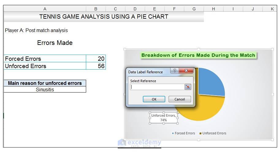
How to Make a Pie Chart in Excel & Add Rich Data Labels to The Chart!

How to create a creative multi-layer Doughnut Chart in Excel The doughnut chart is a better version of the pie chart. While most people still use pie charts when they build reports and dashboards, the doughnut chart is the only reasonable choice for circular charts in a dashboard in my opinion. IMPORTANT: Do not use doughnut charts if you have a big amount of data points to display. A recommended amount ...

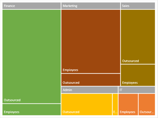
New, better alternative to Pie Charts: Treemap - Efficiency 365

Is there a way to change the order of Data Labels ... Answer. I got your meaning. Please try to double click the the part of the label value, and choose the one you want to show to change the order. * Beware of scammers posting fake support numbers here. * Once complete conversation about this topic, kindly Mark and Vote any replies to benefit others reading this thread.

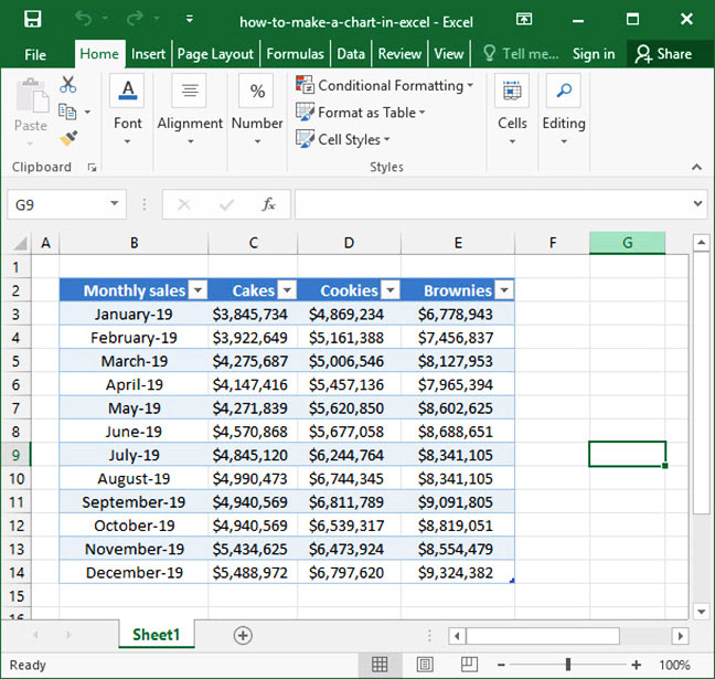
How To Make a Chart In Excel | Deskbright

Adding rich data labels to charts in Excel 2013 ... Putting a data label into a shape can add another type of visual emphasis. To add a data label in a shape, select the data point of interest, then right-click it to pull up the context menu. Click Add Data Label, then click Add Data Callout . The result is that your data label will appear in a graphical callout.

How to Setup a Pie Chart with no Overlapping Labels | Telerik Reporting

Everything You Need to Know About Pie Chart in Excel How to Make a Pie Chart in Excel. Start with selecting your data in Excel. If you include data labels in your selection, Excel will automatically assign them to each column and generate the chart. Go to the INSERT tab in the Ribbon and click on the Pie Chart icon to see the pie chart types. Click on the desired chart to insert.

Advanced Graphs Using Excel : 3D-histogram in Excel

How to fix wrapped data labels in a pie chart | Sage ... Right click on the data label and select Format Data Labels. 2. Select Text Options > Text Box > and un-select Wrap text in shape. 3. The data labels resize to fit all the text on one line. 4. Alternatively, by double-clicking a data label, the handles can be used to resize the label to wrap words as desired. This can be done on all data labels ...

Share :