42 conditional formatting pivot table row labels
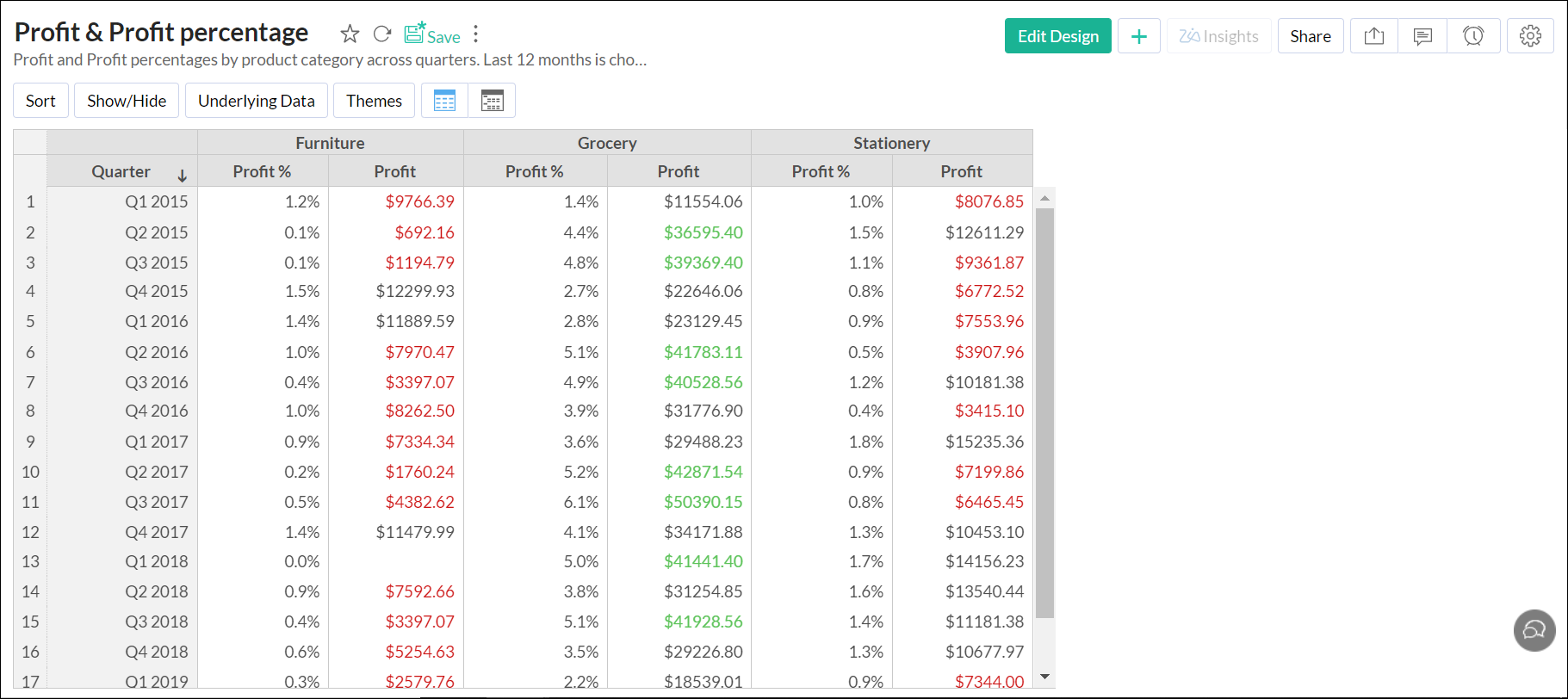
How to make row labels on same line in pivot table? - ExtendOffice Make row labels on same line with PivotTable Options You can also go to the PivotTable Options dialog box to set an option to finish this operation. 1. Click any one cell in the pivot table, and right click to choose PivotTable Options, see screenshot: 2. Add Pivot Table Conditional Formatting and Fix Problems To apply simple conditional formatting: In the pivot table, select the territory sales amounts, in cells B5:C16. On the Ribbon's Home tab, click Conditional Formatting. Click Top/Bottom Rules, and click Above Average. In the Above Average window, select one of the formatting options from the drop down list.
Format Pivot Table Labels Based on Date Range In the pivot table, remove any filters that have been applied - all the rows need to be visible before you apply the conditional formatting. Select all the dates in the Row Labels that you want to format. On the Ribbon, click the Home tab, and then in the Styles group, click Conditional Formatting.

Conditional formatting pivot table row labels
Conditional Formatting in Pivot Table - WallStreetMojo We must follow the steps to apply conditional formatting in the pivot table. First, we must select the data. Then, in the "Insert" Tab, click on "Pivot Tables." As a result, a dialog box appears. Next, we must insert the pivot table in a new worksheet by clicking "OK." Currently, a pivot table is blank. Next, we need to bring in the values. Re-Apply Pivot Table Conditional Formatting - yoursumbuddy This method relies on all the conditional formatting you want to re-apply being in that first row labels cell. In cases where the conditional formatting might not apply to the leftmost row label, I've still applied it to that column, but modified the condition to check which column it's in. This function can be modified and called from a ... Excel VBA: Conditional Format of Pivot Table based on Column Label ... myPivotSourceName = myPivotField.Name. Then rather than referencing the data field with the pivot field object, I referenced the DataRange with the string: myPivotTable.PivotFields (myPivotSourceName).DataRange.Select. Works perfectly and is completely portable for any pivottable on any sheet with any fields. excel vba.
Conditional formatting pivot table row labels. Conditional Formatting in Pivot Table (Example) | How To Apply? - EDUCBA Click on any cell in the pivot table > Go to the HOME tab > Click on Conditional Formatting option under Styles option > Click on Manage Rules option. It will open a Rules Manager dialog box. Click on the Edit Rule tab, as shown in the below screenshot. It will open the Editing Rule formatting window. Refer to the below screenshot. Conditional formatting rows in a pivot table based on one rows criteria ... I am havong difficulty trying to highlight an entire row in a pivot table based on one rows criteria. The pivot table is from A:M and I need to highlight the corresponding row if column I has 992 in it. I have tried sevral ways but can only get it to work if I just focus on one row. I am at a loss for what I am doing wrong. How to Format Excel Pivot Table - Contextures Excel Tips First, select a cell in the pivot table. Next, on the Excel Ribbon, click the Design tab. In the PivotTable Styles gallery, scroll to the bottom. Click the New PivotTable Style command. Next, follow the steps in the next section below, to name and modify the new style. Pivot Table Conditional Formatting for Different Rows Items? Hello, It is possible! All you have to do: Select Your Pivot Table and: Go to Conditional Formatting -> New Rule -> Choose All cells showing "duration" values for "Type and "Date Selection" under "Apply Rule To" section -> Use a Formula to Determine which cells to format and enter the following formula: =AND(A6="Cars",A6>3), You can create new rules for other two conditions as well:
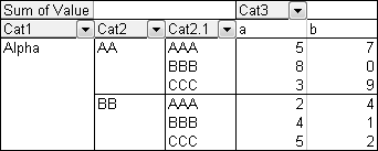
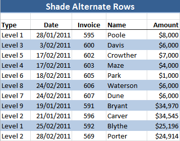
Conditional Formatting in a Pivot Table - MrExcel Message Board Those 3 scoping options are the ones described in the Microsoft link I referenced. Add, change, find, or clear conditional formats - Excel - Office.com. The step of: Home>Styles>Conditional Formatting>Manage Rules. Once here, there is a drop down at the top of the dialog box: "Show formatting rules for :". Conditional Formatting PivotTables - My Online Training Hub Here's a step by step how to: 1. Select any cell in the values area of your PivotTable. 2. On the Home tab of the Ribbon select Conditional Formatting > Top/Bottom Rules > Top 10 Items: 3. Set the value to 1 and choose your format: 4. You will now have an icon beside the cell that you have applied the formatting to. Apply Conditional Formatting | Excel Pivot Table Tutorial - Excel Champs First of all, select any of the cells which have month value. Then, go to Home Tab → Styles → Conditional Formatting → New Rule. Here, you will get a pop-up window to apply conditional formatting to the pivot table. In this pop-up window, you have three different options to apply conditional formatting in pivot table. Conditional formatting of pivot table by row label Conditional formatting of pivot table by row label. I would like to format my pivot table so that the alternative row labels are highlighted when the table is in tabular format. Here is an example of the desired formatting: New Bitmap Image.jpg. Thanks in advance!
Pivot Table Grouping, Ungrouping And Conditional Formatting #1) Select the entire column under the Sum of Total column in the pivot table. #2) Navigate to Home -> Conditional Formatting #3) Select Top/Bottom Rules -> Bottom 10 items. #4) In the dialog reduce the count to 3 (since we want just the bottom 3) and you can choose any highlighter from the drop-down. How to Apply Conditional Formatting to Pivot Tables So in this post I explain how to apply conditional formatting for pivot tables. 1. Select a cell in the Values area The first step is to select a cell in the Values area of the pivot table. If your pivot table has multiple fields in the Values area, select a cell for the field you want to apply the formatting to. 2. Apply Conditional Formatting conditional formatting per row on pivot - Microsoft Tech Community conditional formatting per row on pivot. I would like to format each row of a pivot table separately (as in the picture shown below), but I cannot paste the formatting. I've got many rows, and they could change (just like the columns) Is there a way to automate this, or I have to select row by row and apply the formatting? Design the layout and format of a PivotTable - support.microsoft.com Right-click the field name and then select the appropriate command — Add to Report Filter, Add to Column Label, Add to Row Label, or Add to Values — to place the field in a specific area of the layout section. Click and hold a field name, and then drag the field between the field section and an area in the layout section.
How to Sort Pivot Table Row Labels, Column Field Labels and Data Values with Excel VBA Macro ...
Excel Pivot Table Conditional Formatting Row Labels Go making the conditional formatting select the color scale and do it based on commercial and choose diverging and the colors should give expected result. Here a glaze color or bar and been applied...
Pivot Table Conditional Formatting with VBA - Peltier Tech Blog
Overwrite pivot table conditional format based on row label As far as I know, using the one rule in the Conditional formatting, we can only format the cells with one color if the condition is true and if the same condition is false, the formatting of the cell will be blank and if both conditions are true, the formatting of cell depends on the highest ranking/priority of the rules in Conditional formatting.

How to use Conditional Formatting in the Pivot table | Excelinexcel
Conditional formatting for Pivot Tables in Excel 2016 - 2007 - Ablebits Conditional formatting when applied to PivotTables in Excel 2007 - 2016 is applied to the underlying structure of the PivotTable rather than to the cells themselves. So, when you interact with a PivotTable such as moving fields around and viewing your data in different ways, the formatting is updated as you work.

microsoft office - Excel 2013 table formatting - Super User
Pivot Table Conditional Formatting - Microsoft Tech Community Hi all :) I have an issue conditionally formatting a Pivot Table. I have my row hierarchy set up as Region, Area, Store, Consultant. My rows are expanded out only to a Store Level. I need the Store Name to be highlighted red if the value in the first column is <1. I have applied conditional fo...

How to Sort Pivot Table Row Labels, Column Field Labels and Data Values with Excel VBA Macro ...
Pivot Table: Pivot table conditional formatting - Exceljet Select any cell in the data you wish to format and then choose "New rule" from the conditional formatting menu on the Home tab of the ribbon. At the top of the window, you will see setting for which cells to apply conditional formatting to. For the example shown, we want: "All cells showing sum of "sales values" for name and "date"

How To Find And Remove Duplicates In A Pivot Table - MS Excel | Excel In Excel
Pivot Table Conditional Formatting with VBA - Peltier Tech sub formatpt1 () dim c as range with activesheet.pivottables ("pivottable1") ' reset default formatting with .tablerange1 .font.bold = false .interior.colorindex = 0 end with ' apply formatting to each row if condition is met for each c in .databodyrange.cells if c.value >= 7 then with .tablerange1.rows (c.row - .tablerange1.row + 1) …
Customizing Pivot Table | Zoho Analytics On-Premise
How to Apply Conditional Formatting to Rows Based on Cell Value On the Home tab of the Ribbon, select the Conditional Formatting drop-down and click on Manage Rules…. That will bring up the Conditional Formatting Rules Manager window. Click on New Rule. This will open the New Formatting Rule window. Under Select a Rule Type, choose Use a formula to determine which cells to format.

Conditional Formatting
Conditional Format Pivot Table Row - Chandoo.org Select the entire row, and when you apply the conditional format, make the column reference absolute. So, say we want the entire row 2 to be formatted if cell in col B = 5. formula would be: =$B2=5
Formatting Tips for Pivot Tables - Goodly
How to rename group or row labels in Excel PivotTable? - ExtendOffice To rename Row Labels, you need to go to the Active Field textbox. 1. Click at the PivotTable, then click Analyze tab and go to the Active Field textbox. 2. Now in the Active Field textbox, the active field name is displayed, you can change it in the textbox. You can change other Row Labels name by clicking the relative fields in the PivotTable ...
Conditional Formatting in Pivot Table (Example) | How To Apply?
Excel VBA: Conditional Format of Pivot Table based on Column Label ... myPivotSourceName = myPivotField.Name. Then rather than referencing the data field with the pivot field object, I referenced the DataRange with the string: myPivotTable.PivotFields (myPivotSourceName).DataRange.Select. Works perfectly and is completely portable for any pivottable on any sheet with any fields. excel vba.
Excel Conditional Formatting Zebra Stripes • My Online Training Hub
Re-Apply Pivot Table Conditional Formatting - yoursumbuddy This method relies on all the conditional formatting you want to re-apply being in that first row labels cell. In cases where the conditional formatting might not apply to the leftmost row label, I've still applied it to that column, but modified the condition to check which column it's in. This function can be modified and called from a ...
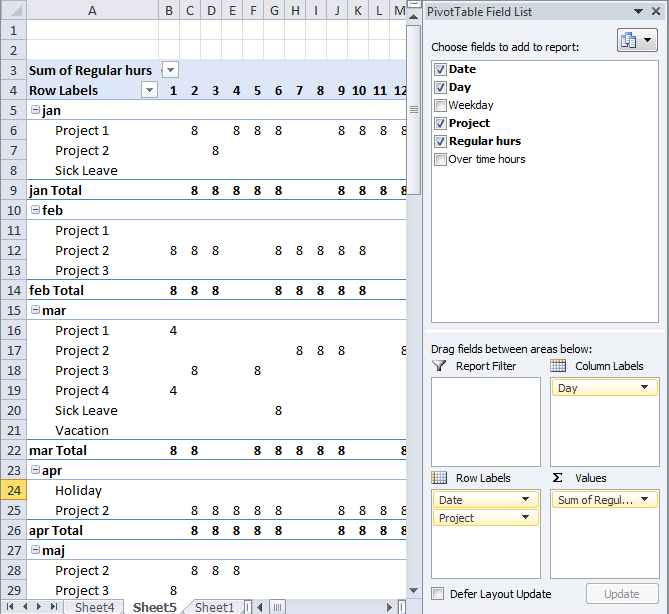
Monthly time sheet by project
Conditional Formatting in Pivot Table - WallStreetMojo We must follow the steps to apply conditional formatting in the pivot table. First, we must select the data. Then, in the "Insert" Tab, click on "Pivot Tables." As a result, a dialog box appears. Next, we must insert the pivot table in a new worksheet by clicking "OK." Currently, a pivot table is blank. Next, we need to bring in the values.
![How to Apply Conditional Formatting to a Pivot Table + [5 Examples]](https://mk0excelchampsdrbkeu.kinstacdn.com/wp-content/uploads/2016/06/Highlght-Top-Values-From-A-Row-By-Using-Conditional-Formatting-In-Pivot-Table-1.png)
How to Apply Conditional Formatting to a Pivot Table + [5 Examples]

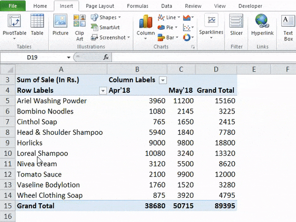
How to Create a MS Excel Pivot Table – An Introduction | SIMPLE TAX INDIA

How to use conditional formatting in decorating pivot tables – Basic Excel Tutorial
33 Pivot Table Blank Row Label - Labels Database 2020
Post a Comment for "42 conditional formatting pivot table row labels"