42 format data labels excel mac

Format Number Options for Chart Data Labels in Excel 2011 for Mac Follow these steps to learn how to format the values used in Data Labels within Excel 2011: Select the chart -- then select the Charts tab which appears on the Ribbon, as shown highlighted in red within Figure 2. Within the Charts tab, click the Edit button (highlighted in blue within Figure 2) to open the Edit menu. Values From Cell: Missing Data Labels Option in Excel 2016? (Mac) For a new thread (1st post), scroll to Manage Attachments, otherwise scroll down to GO ADVANCED, click, and then scroll down to MANAGE ATTACHMENTS and click again. Now follow the instructions at the top of that screen. New Notice for experts and gurus:

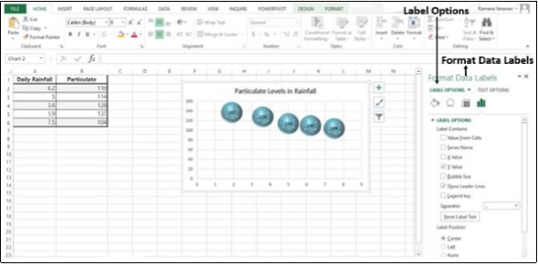
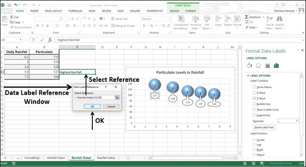
Add or remove data labels in a chart - support.microsoft.com Right-click the data series or data label to display more data for, and then click Format Data Labels. Click Label Options and under Label Contains, select the Values From Cells checkbox. When the Data Label Range dialog box appears, go back to the spreadsheet and select the range for which you want the cell values to display as data labels.

Format data labels excel mac

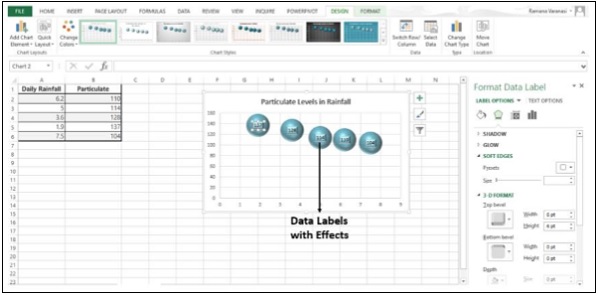
How to Change Excel Chart Data Labels to Custom Values? First add data labels to the chart (Layout Ribbon > Data Labels) Define the new data label values in a bunch of cells, like this: Now, click on any data label. This will select "all" data labels. Now click once again. At this point excel will select only one data label. Go to Formula bar, press = and point to the cell where the data label ... Change the format of data labels in a chart To get there, after adding your data labels, select the data label to format, and then click Chart Elements > Data Labels > More Options. To go to the appropriate area, click one of the four icons ( Fill & Line, Effects, Size & Properties ( Layout & Properties in Outlook or Word), or Label Options) shown here. How to add data labels from different column in an Excel chart? This method will introduce a solution to add all data labels from a different column in an Excel chart at the same time. Please do as follows: 1. Right click the data series in the chart, and select Add Data Labels > Add Data Labels from the context menu to add data labels. 2. Right click the data series, and select Format Data Labels from the ...

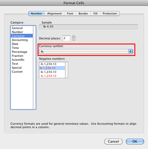
Format data labels excel mac. Modify chart data in Numbers on Mac - Apple Support Click the chart, click Edit Data References, then do any of the following in the table containing the data: Remove a data series: Click the dot for the row or column you want to delete, then press Delete on your keyboard. Add an entire row or column as a data series: Click its header cell. If the row or column doesn't have a header cell, drag ... How to Create Labels in Word from an Excel Spreadsheet Select Browse in the pane on the right. Choose a folder to save your spreadsheet in, enter a name for your spreadsheet in the File name field, and select Save at the bottom of the window. Close the Excel window. Your Excel spreadsheet is now ready. 2. Configure Labels in Word. Mac: XAxis data label format issue excel chart The reports with the X and Y axis values are populating correctly in Windows, where as in Mac environment the X-axis values are showing special characters in the data labels/ticker labels i.e. eg: if the data label name is "1-Year Profit Margin" it is showing as "$1-Year Profit Margin". How to format the data labels in Excel:Mac 2011 when showing a ... Phillip M Jones Replied on December 7, 2015 Try clicking on Column or Row you want to set. Go to Format Menu Click cells Click on Currency Change number of places to 0 (zero) (if in accounting do the same thing. _________ Disclaimer:

How to Add Axis Labels in Excel Charts - Step-by-Step (2022) Left-click the Excel chart. 2. Click the plus button in the upper right corner of the chart. 3. Click Axis Titles to put a checkmark in the axis title checkbox. This will display axis titles. 4. Click the added axis title text box to write your axis label. Or you can go to the 'Chart Design' tab, and click the 'Add Chart Element' button ... How to Print Labels from Excel - Lifewire Choose Start Mail Merge > Labels . Choose the brand in the Label Vendors box and then choose the product number, which is listed on the label package. You can also select New Label if you want to enter custom label dimensions. Click OK when you are ready to proceed. Connect the Worksheet to the Labels Change the look of chart text and labels in Numbers on Mac Change the look of chart text and labels in Numbers on Mac You can change the look of chart text by applying a different style to it, changing its font, adding a border, and more. If you can't edit a chart, you may need to unlock it. Change the font, style, and size of chart text Edit the chart title Add and modify chart value labels Format Trendlines in Excel Charts - Instructions and Video Lesson To format trendlines in Excel, click the "Format" tab within the "Chart Tools" contextual tab in the Ribbon. Then select a trendline to format from the "Chart Elements" drop-down in the "Current Selection" button group. Then click the "Format Selection" button that appears below the drop-down menu in the same area.

How to Print Labels From Excel - EDUCBA Select the file in which the labels are stored and click Open. A new pop up box named Confirm Data Source will appear. Click on OK to let the system know that you want to use the data source. Again a pop-up window named Select Table will appear. Click on OK to select the table from your excel sheet for labels. Step #5 - Add Mail Merge Fields Problems formatting pivot chart data labels in Mac v16 Clicking a single data label. All the Excel documentation suggests that selecting a single data label should select ALL data labels; only a second click will select just that single label With the pivot chart selected, on the ribbon choose Add Chart Element > Data Labels > More Data Label Options How to Create Mailing Labels in Excel - Excelchat Step 1 - Prepare Address list for making labels in Excel First, we will enter the headings for our list in the manner as seen below. First Name Last Name Street Address City State ZIP Code Figure 2 - Headers for mail merge Tip: Rather than create a single name column, split into small pieces for title, first name, middle name, last name. How Do I Create Avery Labels From Excel? - Ink Saver Arrange the fields: Next, arrange the columns and rows in the order they appear in your label. This step is optional but highly recommended if your designs look neat. For this, just double click or drag and drop them in the text box on your right. Don't forget to add commas and spaces to separate fields

Use Excel PivotTables to quickly analyze grades - Extra Credit

Prevent Overlapping Data Labels in Excel Charts - Peltier Tech _ datalabels (ipoint) if firstlabel.top + firstlabel.height * (1 - overlaptolerance) > _ secondlabel.top then didnotoverlap = false firstlabel.top = firstlabel.top - moveincrement secondlabel.top = secondlabel.top + moveincrement end if end if next end if next if didnotoverlap then exit do dim loopcounter as long loopcounter = …

GNIIT HELP: Advanced Excel - Richer Data Labels ~ GNIITHELP

How to Print Address Labels From Excel? (with Examples) First, select the list of addresses in the Excel sheet, including the header. Go to the "Formulas" tab and select "Define Name" under the group "Defined Names.". A dialog box called a new name is opened. Give a name and click on "OK" to close the box. Step 2: Create the mail merge document in the Microsoft word.

Do My Excel Blog: How to hide the zero percent labels in an Excel pie chart

Format Data Labels in Excel- Instructions - TeachUcomp, Inc. To do this, click the "Format" tab within the "Chart Tools" contextual tab in the Ribbon. Then select the data labels to format from the "Chart Elements" drop-down in the "Current Selection" button group. Then click the "Format Selection" button that appears below the drop-down menu in the same area.

Microsoft Excel Tutorials: Add Data Labels to a Pie Chart

How to change chart axis labels' font color and size in Excel? Just click to select the axis you will change all labels' font color and size in the chart, and then type a font size into the Font Size box, click the Font color button and specify a font color from the drop down list in the Font group on the Home tab. See below screen shot:

Excel Custom Chart Labels • My Online Training Hub

Excel tutorial: The Format Task pane This will open the Format Task Pane with Chart Options selected. You can also select a chart element first, then use the keyboard shortcut Control + 1. For example, if I select the data bars in this chart, then type Control + 1, the Format Task Pane will open with with the data series options selected.

31 What Is A Category Label In Excel - Labels Database 2020

format data labels Excel | Excelchat - GICRM AI Place the upper-left corner of the chart inside cell I22. Format the Legend of the chart to appear at the bottom of the chart area. Format the Data Labels to appear on the Outside end of the chart. Note, Mac users, select the range I18:J20, on the Insert tab, click Recommended Charts, and then click Pie.

Fit more text in column headings - Excel for Mac

Formatting data labels and printing pie charts on Excel for Mac 2019 ... Here's a work around I found for printing pie charts. Still can't find a solution for formatting the data labels. 1. When printing a pie chart from Excel for mac 2019, MS instructions are to select the chart only, on the worksheet > file > print. Excel is supposed to print the chart only (not the data ) and automatically fit it onto one page.

Format data labels in a chart in Office 2016 for Mac - Office Support

Move and Align Chart Titles, Labels, Legends with the ... - Excel Campus Select the element in the chart you want to move (title, data labels, legend, plot area). On the add-in window press the "Move Selected Object with Arrow Keys" button. This is a toggle button and you want to press it down to turn on the arrow keys. Press any of the arrow keys on the keyboard to move the chart element.

Advanced Excel - более богатые метки данных - CoderLessons.com

Format Number Options for Chart Data Labels in PowerPoint 2011 for Mac Figure 2: Select the Data Label Options. Alternatively, select the Data Labels for a Data Series in your chart and right-click ( Ctrl +click) to bring up a contextual menu -- from this menu, choose the Format Data Labels option as shown in Figure 3 . Figure 3: Select the Format Data Labels option. Either of the above options will summon the ...

Format Data Labels in Excel- Instructions - TeachUcomp, Inc.

How to Create Address Labels from Excel on PC or Mac menu, select All Apps, open Microsoft Office, then click Microsoft Excel. If you have a Mac, open the Launchpad, then click Microsoft Excel. It may be in a folder called Microsoft Office. 2 Enter field names for each column on the first row. The first row in the sheet must contain header for each type of data. [1]

Format Number Options for Chart Data Labels in Excel 2011 for Mac

How to add data labels from different column in an Excel chart? This method will introduce a solution to add all data labels from a different column in an Excel chart at the same time. Please do as follows: 1. Right click the data series in the chart, and select Add Data Labels > Add Data Labels from the context menu to add data labels. 2. Right click the data series, and select Format Data Labels from the ...

How to Add Data Labels in Excel - Excelchat | Excelchat

Change the format of data labels in a chart To get there, after adding your data labels, select the data label to format, and then click Chart Elements > Data Labels > More Options. To go to the appropriate area, click one of the four icons ( Fill & Line, Effects, Size & Properties ( Layout & Properties in Outlook or Word), or Label Options) shown here.